For many new and aspiring data scientists, linear regression is most likely the first machine learning model everyone learns. It’s pretty intuitive and straightforward to understand. After all, it starts with a familiar formula where y = mx + b; most likely, most folks have seen it during high school or university.
Even though it is a popular model, aspiring data scientists often misuse the model because they do not check if the underlying model’s assumptions are true.
In this article, I’ll be going over the assumptions of linear regression, how to check them, and how to interpret them - techniques to use if the assumptions are not met. I’m assuming you’ll have a basic understanding of the OLS linear regression model.
The 4 Key assumptions are:
- Linearity There is a linear relationship between the independent and dependent variables.
- Independence
- Each observation is independent of one another.
- Homoscedasticity
- The variance of the errors is constant across different independent variables.
- Normality
- The errors are normally distributed and are centered around zero.
Checking the 1st assumption: Linearity between the X and Y.
To check this assumption, it’s pretty easy. Create a scatter plot with X and Y.
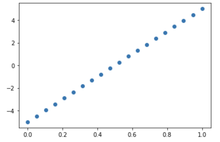
If you see something like the plot above, you can safely assume your X and Y have a linear relationship. It doesn’t have to be perfect like the plot above, as long as you can visually conclude there is some sort of linear relationship.
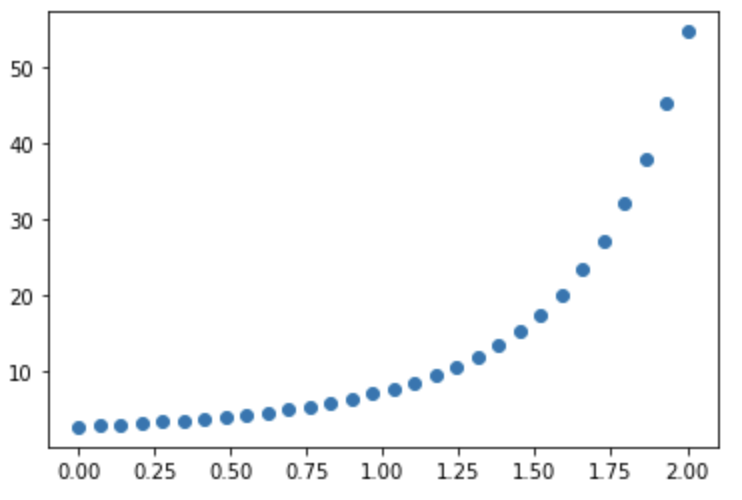
The plot above does have a relationship, but it is not linear. It has somewhat a polynomial relationship instead. If identified, you may have to encode new features to capture the non-linear relationship in your linear regression.
However, if the assumption above is not true, you can employ a couple of strategies.
-
You may want to employ a polynomial transformation to the independent variable if a relationship is not linear.
-
You may want to apply a nonlinear transformation. You may want to take a log or the square root as typical examples.
Assumption 2: Independence of each observation
This means that a residual of an observation should not predict the next observation.
For the most part, if we’re working with non-time-series data, and each observation is independent, and we have an understanding of how our data is collected, then this assumption is generally satisfied. However, domain knowledge is essential in making assumptions if you don’t know how the data is collected.
Plot a residual in time order; you want to see randomness.
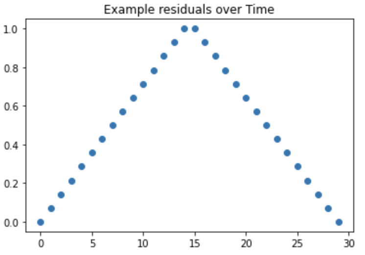
The above plot is something you do not want to see. There is an obvious pattern and no randomness.
Assumption 3: The residuals are homoskedastic (not heteroscedastic)
First, let’s define what homoscedastic means? It refers to the variance of the error to be constant on all data points of X. For example, an X value of 7-9 should not have a higher variance in the error term than the X value between 1-3. It’s best understood to visualize, and it’s an excellent habit to visualize your residuals when performing your linear regression.
Heteroscedasticity can occur in a few ways, but most commonly, it occurs when the error variance changes proportionally with a factor. Here’s a good example taken from Jim Frost’s article on hetroscedasticity in linear regression.
Suppose you were to model consumption based on income. You’ll identify that the variability in consumption increases as income increases. Individuals with lower income will have less variability since there is little room for other spending besides necessities. Folks with higher income have more disposable income on luxury items, which may result in a broader spread of spending habits.
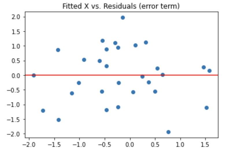
The above plot is an example of the residuals being homoskedastic. There is visible randomness and no discerning patterns recognized.
If our residuals are not homoskedastic, we can try a few things.
-
The easiest thing you can do is try another regression model, such as the weighted least squares model, which will fix the heteroscedasticity.
-
You may try to redefine the independent variable.
-
You may try transforming the dependent variable; however, this will lead to difficulties in interpreting the results.
Assumption 4: Our residuals are normally distributed.
The easiest way to check this is to plot a histogram on your residuals or employ a Q-Q plot.
Alternatively, we can also employ a Q-Q plot, which also helps us visually determine if our residuals follow a normal distribution.
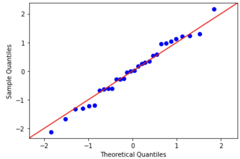
The closer the residuals follow the line, the more normal the distribution is. However, if you notice there is a skew in your residuals. A log transformation on your dependent variable may help. However, this does result in difficulties of interpreting your result.
Other things you may want to check
Overall, before doing a linear regression analysis, you may want to do a few things. Such as:
- Checking and removing outliers
- Scaling your data (especially with multivariate linear regression)
- Check and reduce Multicollinearity in multivariate linear regression.
- It is also worth considering using a generalized linear model (GLM) instead of the classical OLS linear regression.
From a data science point of view, at the end of the day. Models are mainly accessed on how well they perform. If your main goal is to build a robust predictor well, then checking for these assumptions may not be as important. However, validating these assumptions is important if you’re focused on statistical inference.
Resources:
- An Introduction to Statistical Learning - Gareth James, Daniela Witten, Trevor Hastie, Robert Tibshirani
- https://www.statology.org/linear-regression-assumptions/
- Regression Anlaysis by Jim Frost