Using Latent Dirichlet Allocation (LDA) and Non-negative Matrix Factorization (NMF) topic modelling methods
Every time I read an article from the New York Times, I usually like to read through some of the comments to get a better perspective on a story. However, sometimes there are thousands of comments and I don’t have time to read through them all and would like to get the gist of the main discussion points.
Setting up a quick topic modeling script could help me get the gist of the key topics folks are discussing about in the comment section of an article.
Note: We will be using Latent Dirichlet Allocaiton (LDA) and Non-negative Matrix Factorization(NMF) methods in this tutorial. I won’t go in-depth into explaining how it works, as there are many great articles on medium discussing this. This is strictly a programming tutorial to get your topic modeling code set up quickly.
Step 1: Collecting the comments
I will be analyzing the comment section from this New York Times’ article.
I published a medium post last week on how to collect comments from a New York Times article. Please follow that tutorial first, before continuing on with this one.
Step 2: Setting things up
#Importing Required Plugins
import pandas as pd
import numpy as np#load csv file to Pandas Dataframe
df = pd.read_csv('nyt_comments.csv', index_col = 0)
If you followed my tutorial from this medium post, your dataframe should look something like this.

Step 3: Pre-processing the text data.
For topic modeling the data type we are using is text data, and it will require some form of pre-processing in order to make the results a little cleaner.
During the pre-processing stage, usually:
set all words to lowercase
remove punctuation
removing stopwords (and, the, etc.)
reducing the words to their root form, this is called stemming.
Note: I’m using the SnowballStemmer in my script below, however you can use any other stemmer.
from nltk.stem.snowball import SnowballStemmer
from nltk.corpus import stopwords
import string

stop_words = stopwords.words('english')
def tokenizer(text):
    '''
    -covert everything to lowercase
    -remove punctuations
    -remove stopwords
    -stemmer
    '''
    #All characters in this string will be converted to lowercase
    text = text.lower()

    #Removing sentence punctuations
    for punctuation_mark in string.punctuation:
        text = text.replace(punctuation_mark,'')

    #Creating our list of tokens
    list_of_tokens = text.split(' ')
    #Creating our cleaned tokens list
    cleaned_tokens = []
    #Let us use a stemmer
    stemmer = SnowballStemmer(language = 'english')

    #Removing Stop Words in our list of tokens and any tokens that happens to be empty strings
    for token in list_of_tokens:
        if (not token in stop_words) and (token != ''):
            #Stem tokens
            token_stemmed = stemmer.stem(token)
            #appending our finalized cleaned token
            cleaned_tokens.append(token_stemmed)

    return cleaned_tokens
Step 4: Using the Sklearn’s TfidfVectorizer to covert our text data into term-frequency inverse document matrix
from sklearn.feature_extraction.text import TfidfVectorizer
#Instatiate TFIDF Vectorizer
tfidf = TfidfVectorizer(tokenizer = tokenizer,
                           min_df = 0.05,
                           ngram_range = (1,3))

#df.commentBody is referring to the text column from my dataframe containing the comments
token_matrix = tfidf.fit_transform(df.commentBody)

#If you would like to store the matrix to a dataframe, execute the code below
matrix_df = pd.DataFrame(token_matrix.toarray(),
                        columns = tfidf.get_feature_names())
The tf–idf value increases proportionally to the number of times a word appears in the document and is offset by the number of documents in the corpus that contain the word, which helps to adjust for the fact that some words appear more frequently in general. — Wikepedia
Note: You can set the min_df on our TfidfVectorizer to whatever you like, however I chose 0.05 as it seemed to work well on my run of the data.
Step 5: Topic Modeling using LDA
#Import LDA topic modelling plugin from sklearn
from sklearn.decomposition import LatentDirichletAllocation as LDA

#I want 15 topics generated
num_topics = 15

#instatiate LDA model
lda_model = LDA(n_components = num_topics, n_jobs = -1)
lda_model.fit(token_matrix)

#I'm looking for the top 15 words for each topic
top_n_words = 15
token_names = tfidf.get_feature_names()

for topic_num, topic in enumerate(lda_model.components_):
    top_tokens = [token_names[i] for i in topic.argsort()][::-1][:top_n_words] #Returns the indices that would sort an array
    top_n = ', '.join(top_tokens)
    print(f'Topic {topic_num}: {top_n}')
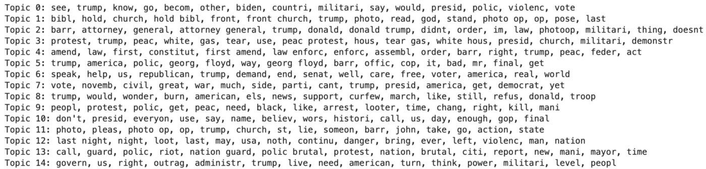
We can clearly identify some of the interesting topic of conversations in the comment section of this article.
However, I wonder if we could get a little bit more context if we took the top 25 words instead of the top 15.
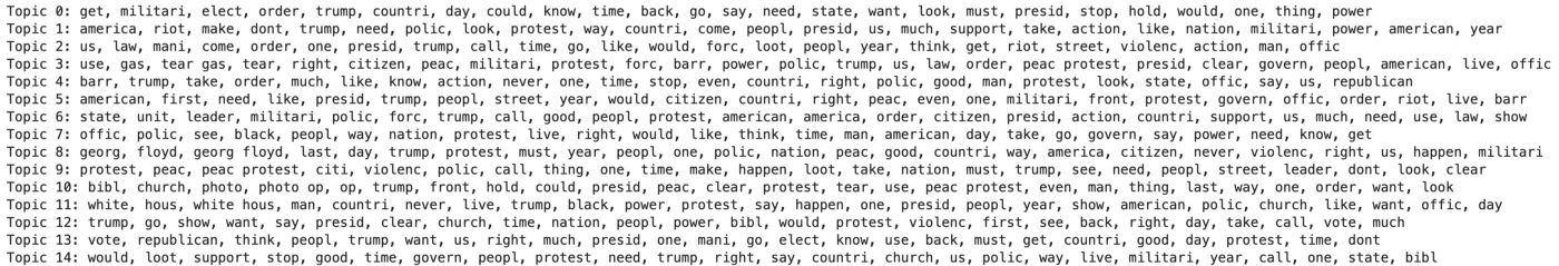
It’s a little bit better in terms of our understanding of the various topics.
Another step we could have taken instead of just increasing the display of top words, is by increasing or decreasing the number of topics our model searches for.
This is where our creative minds are needed, in the input of analyzing the results of our model.
However, let’s take a quick peak into what happens when we decrease the number of topics generated to 10.
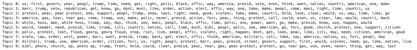
It looks like fewer topics generated do a better job at distinguishing different topics in the comment section of an article.
However, some of the topics don’t really make sense or it is telling us the same thing. This may be due to that these comments are discussing about a specific article already, the topics that can be identified may be limited and that many of the same words are used repeatedly.
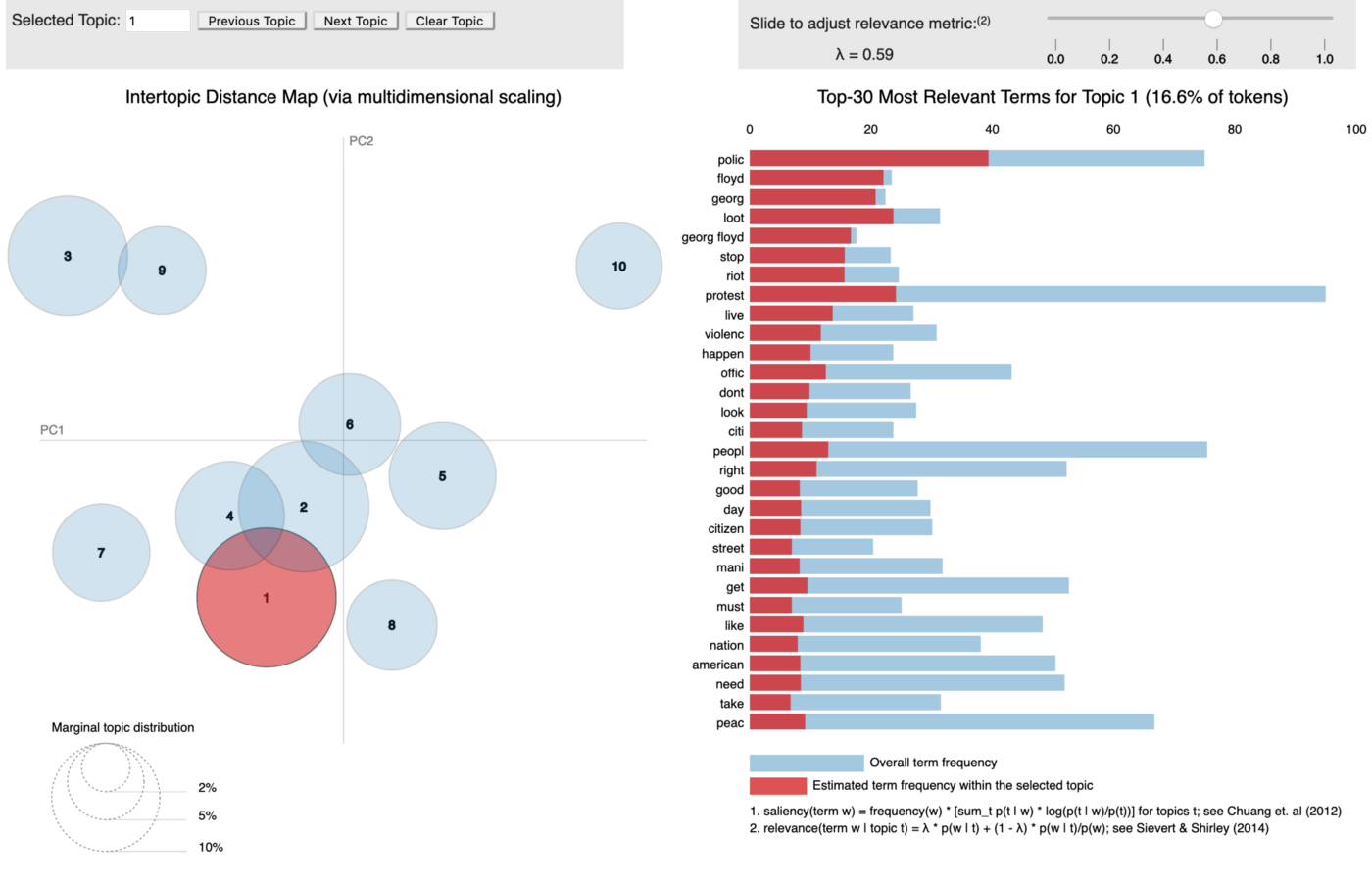
Step 6: Visualizing topics generated by our LDA model with the pyLDAvis plugin
The pyLDAvis plugin generates an interactive plot, which in my opinion makes easier for me in analyzing the various topics generated as well as how well my LDA model performed.
#Import visualization tools for LDA models
import pyLDAvis
import pyLDAvis.sklearn
pyLDAvis.enable_notebook()

# Let us visualize these topics
pyLDAvis.sklearn.prepare(lda_model, token_matrix, tfidf)
Step 7: Topic Modeling with NMF
The setup isn’t entirely to different, quite the same to be honest. However, this algorithm will spit out different results.
from sklearn.decomposition import NMF

#numebr of topics generated
num_topics = 5

#NMF Topic Modeling
NMF_model = NMF(n_components = num_topics)
NMF_model.fit(token_matrix)

#I'm looking for the top 20 words for each topic
top_n_words = 20
token_names = tfidf.get_feature_names()

for topic_num, topic in enumerate(NMF_model.components_):
    top_tokens = [token_names[i] for i in topic.argsort()][::-1][:top_n_words] #Returns the indices that would sort an array
    top_n = ', '.join(top_tokens)

Reducing the number of topics further seems to do an even better job at distinguishing the various topics discussed in the comments.
Note: Unfortunately, you can’t use the pyLDAvis plugin for visualizing topics from the NMF model.
Well, there you go, that is how you would set up a quick script on topic modeling to determine the various topics of discussion within the comment section from a NYT article.